Machine-learning models are growing exponentially larger. At the same time, they require exponentially more energy to train, so that they can accurately process images or text or video. As the AI community grapples with its environmental impact, some conferences now ask paper submitters to include information on CO2 emissions. New research offers a more accurate method for calculating those emissions. It also compares factors that affect them, and tests two methods for reducing them.
Several software packages estimate the carbon emissions of AI workloads. Recently a team at Université Paris-Saclay tested a group of these tools to see if they were reliable. “And they’re not reliable at all,” says Anne-Laure Ligozat, a co-author of that study who was not involved in the new work.
The new approach differs in two respects, says Jesse Dodge, a research scientist at the Allen Institute for AI and the lead author of the new paper, which he presented this week at the ACM Conference on Fairness, Accountability, and Transparency (FAccT). First, it records server chips’ energy usage as a series of measurements, rather than summing their use over the course of training. Second, it aligns this usage data with a series of data points indicating the local emissions per kilowatt-hour (kWh) of energy used. This number also changes continually. “Previous work doesn’t capture a lot of the nuance there,” Dodge says.
The new tool is more sophisticated than older ones but still tracks only some of the energy used in training models. In a preliminary experiment, the team found that a server’s GPUs used 74% of its energy. CPUs and memory used a minority, and they support many workloads simultaneously, so the team focused on GPU usage. They also didn’t measure the energy used to build the computing equipment, or to cool the data center, or to build it and transport engineers to and from the facility. Or the energy used to collect data or run trained models. But the tool provides some guidance on ways to reduce emissions during training.
“What I hope is that the vital first step towards a more green future and more equitable future is transparent reporting,” Dodge says. “Because you can’t improve what you can’t measure.”
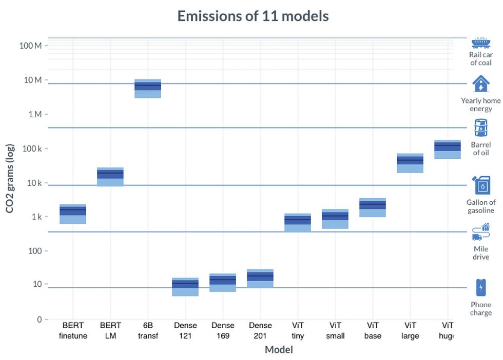
The researchers trained 11 machine-learning models of different sizes to process language or images. Training ranged from an hour on one GPU to eight days on 256 GPUs. They recorded energy used every second or so. They also obtained, for 16 geographical regions, carbon emissions per kWh of energy used throughout 2020, at five-minute granularity. Then they could compare emissions from running different models in different regions at different times.
Powering the GPUs to train the smallest models emitted about as much carbon as charging a phone. The largest model contained six billion parameters, a measure of its size. While training it only to 13% completion, GPUs emitted almost as much carbon as does powering a home for a year. Meanwhile, some deployed models, such as OpenAI’s GPT-3, contain more than 100 billion parameters.
Allen Institute on AI et al from FAccT 2022
The biggest measured factor in reducing emissions was geographical region: Grams of CO2 per kWh ranged from 200 to 755. Besides changing location, the researchers tested two CO2-reduction techniques, allowed by their temporally fine-grained data. The first, Flexible Start, could delay training up to 24 hours. For the largest model, which required several days of training, delaying it up to a day typically reduced emissions less than 1%, but for a much smaller model, such a delay could save 10–80%. The second, Pause and Resume, could pause training at times of high emissions, as long as overall training time didn’t more than double. This method benefited the small model only a few percent, but in half the regions it benefited the largest model 10–30%. Emissions per kWh fluctuate over time in part because, lacking sufficient energy storage, grids must sometimes rely on dirty power sources when intermittent clean sources such as wind and solar can’t meet demand.
Ligozat found these optimization techniques the most interesting part of the paper. But they were based on retrospective data. Dodge says in the future, he’d like to be able to predict emissions per kWh so as to implement them in real time. Ligozat offers another way to reduce emissions: “The first good practice is just to think before running an experiment,” she says. “Be sure that you really need machine learning for your problem.”
Microsoft, whose researchers collaborated on the paper, has already implemented the CO2 metric into its Azure cloud service. Given such information, users might decide to train at different times or in different places, buy carbon offsets, or train a different model or no model at all. “What I hope is that the vital first step towards a more green future and more equitable future is transparent reporting,” Dodge says. “Because you can’t improve what you can’t measure.” Reference: https://ift.tt/YqdGVSb
Dates chiseled into an ancient tombstone have more in common with the data in your phone or laptop than you may realize. They both involve conventional, classical information, carried by hardware that is relatively immune to errors. The situation inside a quantum computer is far different: The information itself has its own idiosyncratic properties, and compared with standard digital microelectronics, state-of-the-art quantum-computer hardware is more than a billion trillion times as likely to suffer a fault. This tremendous susceptibility to errors is the single biggest problem holding back quantum computing from realizing its great promise.
Fortunately, an approach known as quantum error correction (QEC) can remedy this problem, at least in principle. A mature body of theory built up over the past quarter century now provides a solid theoretical foundation, and experimentalists have demonstrated dozens of proof-of-principle examples of QEC. But these experiments still have not reached the level of quality and sophistication needed to reduce the overall error rate in a system.
The two of us, along with many other researchers involved in quantum computing, are trying to move definitively beyond these preliminary demos of QEC so that it can be employed to build useful, large-scale quantum computers. But before describing how we think such error correction can be made practical, we need to first review what makes a quantum computer tick.
Information is physical. This was the mantra of the distinguished IBM researcher Rolf Landauer. Abstract though it may seem, information always involves a physical representation, and the physics matters.
Conventional digital information consists of bits, zeros and ones, which can be represented by classical states of matter, that is, states well described by classical physics. Quantum information, by contrast, involves qubits—quantum bits—whose properties follow the peculiar rules of quantum mechanics.
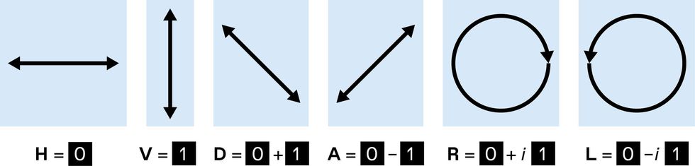
Polarized light is an example of superposition. A classical binary digit could be represented by encoding 0 as horizontally (H) polarized light, and 1 as vertically (V) polarized light. Light polarized at other angles has components of both H and V, representing 0 and 1 simultaneously. Examples include the diagonal (D) polarization at 45°, the antidiagonal (A) at –45°, as well as right (R) and left (L) circularly polarized light (the imaginary number i represents a difference in phase). These states become fully fledged quantum bits (qubits) when they consist of pulses that each contain a single photon.
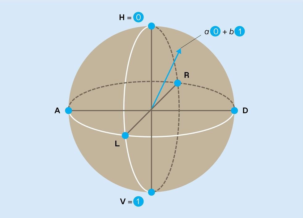
The possible states of a single isolated qubit [blue arrow] are neatly represented on a sphere, known as a Bloch sphere. The states 0 and 1 sit at the north and south poles, and the polarization states D, A, R, and L lie on the equator. Other possible superpositions of 0 and 1 (described by complex numbers a and b) cover the rest of the surface. Noise can make the qubit state wander continuously from its correct location.
A classical bit has only two possible values: 0 or 1. A qubit, however, can occupy a superposition of these two information states, taking on characteristics of both. Polarized light provides intuitive examples of superpositions. You could use horizontally polarized light to represent 0 and vertically polarized light to represent 1, but light can also be polarized on an angle and then has both horizontal and vertical components at once. Indeed, one way to represent a qubit is by the polarization of a single photon of light.
These ideas generalize to groups of n bits or qubits: n bits can represent any one of 2n possible values at any moment, while n qubits can include components corresponding to all 2n classical states simultaneously in superposition. These superpositions provide a vast range of possible states for a quantum computer to work with, albeit with limitations on how they can be manipulated and accessed. Superposition of information is a central resource used in quantum processing and, along with other quantum rules, enables powerful new ways to compute.
Researchers are experimenting with many different physical systems to hold and process quantum information, including light, trapped atoms and ions, and solid-state devices based on semiconductors or superconductors. For the purpose of realizing qubits, all these systems follow the same underlying mathematical rules of quantum physics, and all of them are highly sensitive to environmental fluctuations that introduce errors. By contrast, the transistors that handle classical information in modern digital electronics can reliably perform a billion operations per second for decades with a vanishingly small chance of a hardware fault.
Of particular concern is the fact that qubit states can roam over a continuous range of superpositions. Polarized light again provides a good analogy: The angle of linear polarization can take any value from 0 to 180 degrees.
Pictorially, a qubit’s state can be thought of as an arrow pointing to a location on the surface of a sphere. Known as a Bloch sphere, its north and south poles represent the binary states 0 and 1, respectively, and all other locations on its surface represent possible quantum superpositions of those two states. Noise causes the Bloch arrow to drift around the sphere over time. A conventional computer represents 0 and 1 with physical quantities, such as capacitor voltages, that can be locked near the correct values to suppress this kind of continuous wandering and unwanted bit flips. There is no comparable way to lock the qubit’s “arrow” to its correct location on the Bloch sphere.
Early in the 1990s, Landauer and others argued that this difficulty presented a fundamental obstacle to building useful quantum computers. The issue is known as scalability: Although a simple quantum processor performing a few operations on a handful of qubits might be possible, could you scale up the technology to systems that could run lengthy computations on large arrays of qubits? A type of classical computation called analog computing also uses continuous quantities and is suitable for some tasks, but the problem of continuous errors prevents the complexity of such systems from being scaled up. Continuous errors with qubits seemed to doom quantum computers to the same fate.
We now know better. Theoreticians have successfully adapted the theory of error correction for classical digital data to quantum settings. QEC makes scalable quantum processing possible in a way that is impossible for analog computers. To get a sense of how it works, it’s worthwhile to review how error correction is performed in classical settings.
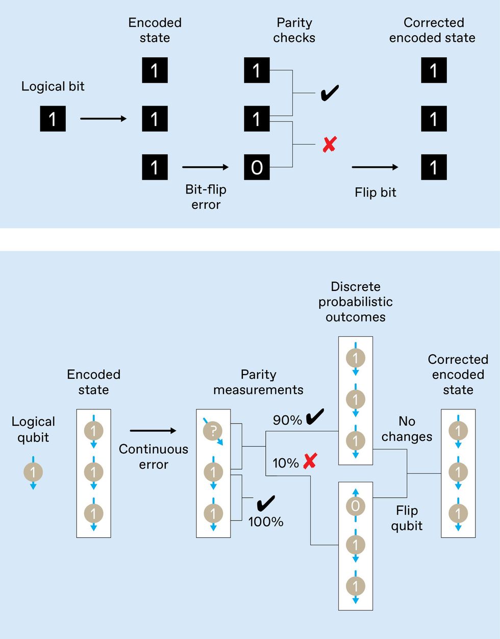
Simple repetition code [top] on a conventional bit allows single bit-flip errors to be detected via parity checks and then corrected. A similar code for qubits [bottom] must deal with continuous errors. (For simplicity, we depict the case of a logical qubit in a nonsuperposition state, 1.) The parity checks, being quantum measurements, produce discrete outcomes with various probabilities, converting the continuous error into a discrete one and allowing correction by a qubit flip. The individual qubit states are not revealed by the parity measurements.
Simple schemes can deal with errors in classical information. For instance, in the 19th century, ships routinely carried clocks for determining the ship’s longitude during voyages. A good clock that could keep track of the time in Greenwich, in combination with the sun’s position in the sky, provided the necessary data. A mistimed clock could lead to dangerous navigational errors, though, so ships often carried at least three of them. Two clocks reading different times could detect when one was at fault, but three were needed to identify which timepiece was faulty and correct it through a majority vote.
The use of multiple clocks is an example of a repetition code: Information is redundantly encoded in multiple physical devices such that a disturbance in one can be identified and corrected.
As you might expect, quantum mechanics adds some major complications when dealing with errors. Two problems in particular might seem to dash any hopes of using a quantum repetition code. The first problem is that measurements fundamentally disturb quantum systems. So if you encoded information on three qubits, for instance, observing them directly to check for errors would ruin them. Like Schrödinger’s cat when its box is opened, their quantum states would be irrevocably changed, spoiling the very quantum features your computer was intended to exploit.
The second issue is a fundamental result in quantum mechanics called the no-cloning theorem, which tells us it is impossible to make a perfect copy of an unknown quantum state. If you know the exact superposition state of your qubit, there is no problem producing any number of other qubits in the same state. But once a computation is running and you no longer know what state a qubit has evolved to, you cannot manufacture faithful copies of that qubit except by duplicating the entire process up to that point.
Fortunately, you can sidestep both of these obstacles. We’ll first describe how to evade the measurement problem using the example of a classical three-bit repetition code. You don’t actually need to know the state of every individual code bit to identify which one, if any, has flipped. Instead, you ask two questions: “Are bits 1 and 2 the same?” and “Are bits 2 and 3 the same?” These are called parity-check questions because two identical bits are said to have even parity, and two unequal bits have odd parity.
The two answers to those questions identify which single bit has flipped, and you can then counterflip that bit to correct the error. You can do all this without ever determining what value each code bit holds. A similar strategy works to correct errors in a quantum system.
Learning the values of the parity checks still requires quantum measurement, but importantly, it does not reveal the underlying quantum information. Additional qubits can be used as disposable resources to obtain the parity values without revealing (and thus without disturbing) the encoded information itself.
Like Schrödinger’s cat when its box is opened, the quantum states of the qubits you measured would be irrevocably changed, spoiling the very quantum features your computer was intended to exploit.
What about no-cloning? It turns out it is possible to take a qubit whose state is unknown and encode that hidden state in a superposition across multiple qubits in a way that does not clone the original information. This process allows you to record what amounts to a single logical qubit of information across three physical qubits, and you can perform parity checks and corrective steps to protect the logical qubit against noise.
Quantum errors consist of more than just bit-flip errors, though, making this simple three-qubit repetition code unsuitable for protecting against all possible quantum errors. True QEC requires something more. That came in the mid-1990s when Peter Shor (then at AT&T Bell Laboratories, in Murray Hill, N.J.) described an elegant scheme to encode one logical qubit into nine physical qubits by embedding a repetition code inside another code. Shor’s scheme protects against an arbitrary quantum error on any one of the physical qubits.
Since then, the QEC community has developed many improved encoding schemes, which use fewer physical qubits per logical qubit—the most compact use five—or enjoy other performance enhancements. Today, the workhorse of large-scale proposals for error correction in quantum computers is called the surface code, developed in the late 1990s by borrowing exotic mathematics from topology and high-energy physics.
It is convenient to think of a quantum computer as being made up of logical qubits and logical gates that sit atop an underlying foundation of physical devices. These physical devices are subject to noise, which creates physical errors that accumulate over time. Periodically, generalized parity measurements (called syndrome measurements) identify the physical errors, and corrections remove them before they cause damage at the logical level.
A quantum computation with QEC then consists of cycles of gates acting on qubits, syndrome measurements, error inference, and corrections. In terms more familiar to engineers, QEC is a form of feedback stabilization that uses indirect measurements to gain just the information needed to correct errors.
QEC is not foolproof, of course. The three-bit repetition code, for example, fails if more than one bit has been flipped. What’s more, the resources and mechanisms that create the encoded quantum states and perform the syndrome measurements are themselves prone to errors. How, then, can a quantum computer perform QEC when all these processes are themselves faulty?
Remarkably, the error-correction cycle can be designed to tolerate errors and faults that occur at every stage, whether in the physical qubits, the physical gates, or even in the very measurements used to infer the existence of errors! Called a fault-tolerant architecture, such a design permits, in principle, error-robust quantum processing even when all the component parts are unreliable.
A long quantum computation will require many cycles of quantum error correction (QEC). Each cycle would consist of gates acting on encoded qubits (performing the computation), followed by syndrome measurements from which errors can be inferred, and corrections. The effectiveness of this QEC feedback loop can be greatly enhanced by including quantum-control techniques (represented by the thick blue outline) to stabilize and optimize each of these processes.
Even in a fault-tolerant architecture, the additional complexity introduces new avenues for failure. The effect of errors is therefore reduced at the logical level only if the underlying physical error rate is not too high. The maximum physical error rate that a specific fault-tolerant architecture can reliably handle is known as its break-even error threshold. If error rates are lower than this threshold, the QEC process tends to suppress errors over the entire cycle. But if error rates exceed the threshold, the added machinery just makes things worse overall.
The theory of fault-tolerant QEC is foundational to every effort to build useful quantum computers because it paves the way to building systems of any size. If QEC is implemented effectively on hardware exceeding certain performance requirements, the effect of errors can be reduced to arbitrarily low levels, enabling the execution of arbitrarily long computations.
At this point, you may be wondering how QEC has evaded the problem of continuous errors, which is fatal for scaling up analog computers. The answer lies in the nature of quantum measurements.
In a typical quantum measurement of a superposition, only a few discrete outcomes are possible, and the physical state changes to match the result that the measurement finds. With the parity-check measurements, this change helps.
Imagine you have a code block of three physical qubits, and one of these qubit states has wandered a little from its ideal state. If you perform a parity measurement, just two results are possible: Most often, the measurement will report the parity state that corresponds to no error, and after the measurement, all three qubits will be in the correct state, whatever it is. Occasionally the measurement will instead indicate the odd parity state, which means an errant qubit is now fully flipped. If so, you can flip that qubit back to restore the desired encoded logical state.
In other words, performing QEC transforms small, continuous errors into infrequent but discrete errors, similar to the errors that arise in digital computers.
Researchers have now demonstrated many of the principles of QEC in the laboratory—from the basics of the repetition code through to complex encodings, logical operations on code words, and repeated cycles of measurement and correction. Current estimates of the break-even threshold for quantum hardware place it at about 1 error in 1,000 operations. This level of performance hasn’t yet been achieved across all the constituent parts of a QEC scheme, but researchers are getting ever closer, achieving multiqubit logic with rates of fewer than about 5 errors per 1,000 operations. Even so, passing that critical milestone will be the beginning of the story, not the end.
On a system with a physical error rate just below the threshold, QEC would require enormous redundancy to push the logical rate down very far. It becomes much less challenging with a physical rate further below the threshold. So just crossing the error threshold is not sufficient—we need to beat it by a wide margin. How can that be done?
A superconducting qubit can be flipped by applying a simple microwave pulse that takes the qubit’s state on a direct path on the Bloch sphere from 0 to 1 [top], but noise will introduce an error in the final position. A complicated pulse producing a more circuitous route can reduce the average amount of error in the final position. Here, the paths are chosen to minimize the effect of noise in the pulse amplitude alone [middle] or in both the amplitude and phase of the pulse [bottom].
If we take a step back, we can see that the challenge of dealing with errors in quantum computers is one of stabilizing a dynamic system against external disturbances. Although the mathematical rules differ for the quantum system, this is a familiar problem in the discipline of control engineering. And just as control theory can help engineers build robots capable of righting themselves when they stumble, quantum-control engineering can suggest the best ways to implement abstract QEC codes on real physical hardware. Quantum control can minimize the effects of noise and make QEC practical.
In essence, quantum control involves optimizing how you implement all the physical processes used in QEC—from individual logic operations to the way measurements are performed. For example, in a system based on superconducting qubits, a qubit is flipped by irradiating it with a microwave pulse. One approach uses a simple type of pulse to move the qubit’s state from one pole of the Bloch sphere, along the Greenwich meridian, to precisely the other pole. Errors arise if the pulse is distorted by noise. It turns out that a more complicated pulse, one that takes the qubit on a well-chosen meandering route from pole to pole, can result in less error in the qubit’s final state under the same noise conditions, even when the new pulse is imperfectly implemented.
One facet of quantum-control engineering involves careful analysis and design of the best pulses for such tasks in a particular imperfect instance of a given system. It is a form of open-loop (measurement-free) control, which complements the closed-loop feedback control used in QEC.
This kind of open-loop control can also change the statistics of the physical-layer errors to better comport with the assumptions of QEC. For example, QEC performance is limited by the worst-case error within a logical block, and individual devices can vary a lot. Reducing that variability is very beneficial. In an experiment our team performed using IBM’s publicly accessible machines, we showed that careful pulse optimization reduced the difference between the best-case and worst-case error in a small group of qubits by more than a factor of 10.
Some error processes arise only while carrying out complex algorithms. For instance, crosstalk errors occur on qubits only when their neighbors are being manipulated. Our team has shown that embedding quantum-control techniques into an algorithm can improve its overall success by orders of magnitude. This technique makes QEC protocols much more likely to correctly identify an error in a physical qubit.
For 25 years, QEC researchers have largely focused on mathematical strategies for encoding qubits and efficiently detecting errors in the encoded sets. Only recently have investigators begun to address the thorny question of how best to implement the full QEC feedback loop in real hardware. And while many areas of QEC technology are ripe for improvement, there is also growing awareness in the community that radical new approaches might be possible by marrying QEC and control theory. One way or another, this approach will turn quantum computing into a reality—and you can carve that in stone.
This article appears in the July 2022 print issue as “Quantum Error Correction at the Threshold.”
Vast surveillance data allows the state to target people whose behavior or characteristics are deemed suspicious by an algorithm, even if they’ve done nothing wrong.
It’s Tuesday night. In front of your house sits a large blue bin, full of newspaper, cardboard, bottles, cans, foil take-out trays, and empty yogurt containers. You may feel virtuous, thinking you’re doing your part to reduce waste. But after you rinse out that yogurt container and toss it into the bin, you probably don’t think much about it ever again.
The truth about recycling in many parts of the United States and much of Europe is sobering. Tomorrow morning, the contents of the recycling bin will be dumped into a truck and taken to the recycling facility to be sorted. Most of the material will head off for processing and eventual use in new products. But a lot of it will end up in a landfill.
So how much of the material that goes into the typical bin avoids a trip to landfill? For countries that do curbside recycling, the number—called the recovery rate—appears to average around 70 to 90 percent, though widespread data isn’t available. That doesn’t seem bad. But in some municipalities, it can go as low as 40 percent.
What’s worse, only a small quantity of all recyclables makes it into the bins—just 32 percent in the United States and 10 to 15 percent globally. That’s a lot of material made from finite resources that needlessly goes to waste.
We have to do better than that. Right now, the recycling industry is facing a financial crisis, thanks to falling prices for sorted recyclables as well as policy, enacted by China in 2018, which restricts the import of many materials destined for recycling and shuts out most recyclables originating in the United States.
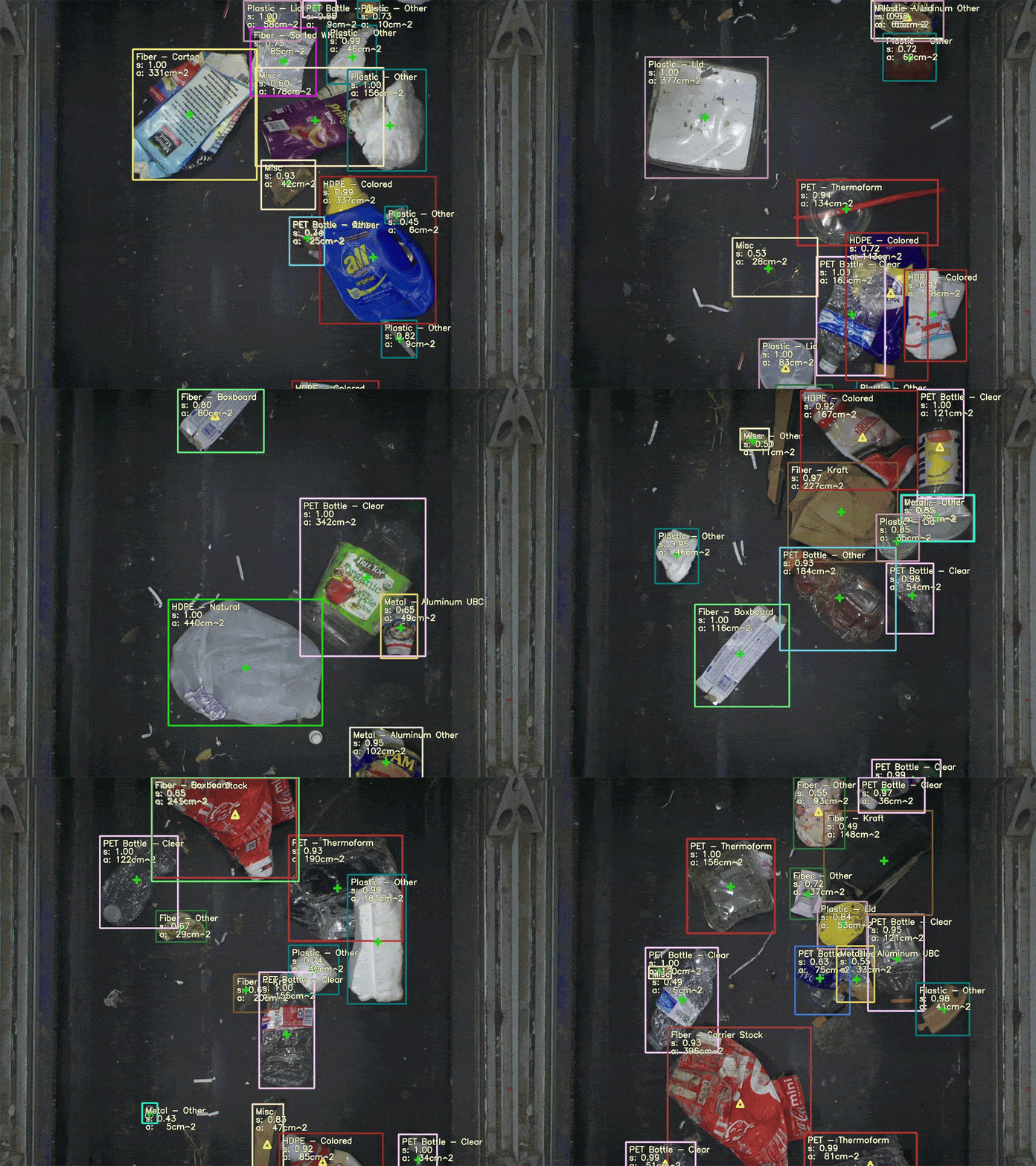
There is a way to do better. Using computer vision, machine learning, and robots to identify and sort recycled material, we can improve the accuracy of automatic sorting machines, reduce the need for human intervention, and boost overall recovery rates.
My company, Amp Robotics, based in Louisville, Colo., is developing hardware and software that relies on image analysis to sort recyclables with far higher accuracy and recovery rates than are typical for conventional systems. Other companies are similarly working to apply AI and robotics to recycling, including Bulk Handling Systems, Machinex, and Tomra. To date, the technology has been installed in hundreds of sorting facilities around the world. Expanding its use will prevent waste and help the environment by keeping recyclables out of landfills and making them easier to reprocess and reuse.
AMP Robotics
Before I explain how AI will improve recycling, let’s look at how recycled materials were sorted in the past and how they’re being sorted in most parts of the world today.
When recycling began in the 1960s, the task of sorting fell to the consumer—newspapers in one bundle, cardboard in another, and glass and cans in their own separate bins. That turned out to be too much of a hassle for many people and limited the amount of recyclable materials gathered.
In the 1970s, many cities took away the multiple bins and replaced them with a single container, with sorting happening downstream. This “single stream” recycling boosted participation, and it is now the dominant form of recycling in developed countries.
Moving the task of sorting further downstream led to the building of sorting facilities. To do the actual sorting, recycling entrepreneurs adapted equipment from the mining and agriculture industries, filling in with human labor as necessary. These sorting systems had no computer intelligence, relying instead on the physical properties of materials to separate them. Glass, for example, can be broken into tiny pieces and then sifted and collected. Cardboard is rigid and light—it can glide over a series of mechanical camlike disks, while other, denser materials fall in between the disks. Ferrous metals can be magnetically separated from other materials; magnetism can also be induced in nonferrous items, like aluminum, using a large eddy current.
By the 1990s, hyperspectral imaging, developed by NASA and first launched in a satellite in 1972, was becoming commercially viable and began to show up in the recycling world. Unlike human eyes, which mostly see in combinations of red, green, and blue, hyperspectral sensors divide images into many more spectral bands. The technology’s ability to distinguish between different types of plastics changed the game for recyclers, bringing not only optical sensing but computer intelligence into the process. Programmable optical sorters were also developed to separate paper products, distinguishing, say, newspaper from junk mail.
So today, much of the sorting is automated. These systems generally sort to 80 to 95 percent purity—that is, 5 to 20 percent of the output shouldn’t be there. For the output to be profitable, however, the purity must be higher than 95 percent; below this threshold, the value drops, and often it’s worth nothing. So humans manually clean up each of the streams, picking out stray objects before the material is compressed and baled for shipping.
Despite all the automated and manual sorting, about 10 to 30 percent of the material that enters the facility ultimately ends up in a landfill. In most cases, more than half of that material is recyclable and worth money but was simply missed.
We’ve pushed the current systems as far as they can go. Only AI can do better.
Getting AI into the recycling businessmeans combining pick-and-place robots with accurate real-time object detection.Pick-and-place robotscombined with computer vision systemsare usedinmanufacturing to grabparticular objects, but they generally are just looking repeatedly for a single item, or for a few items of known shapes and under controlled lighting conditions.Recycling, though, involves infinite variability in the kinds, shapes, and orientations of the objects traveling down the conveyor belt, requiring nearly instantaneous identification along with the quick dispatch of a new trajectory to the robot arm.
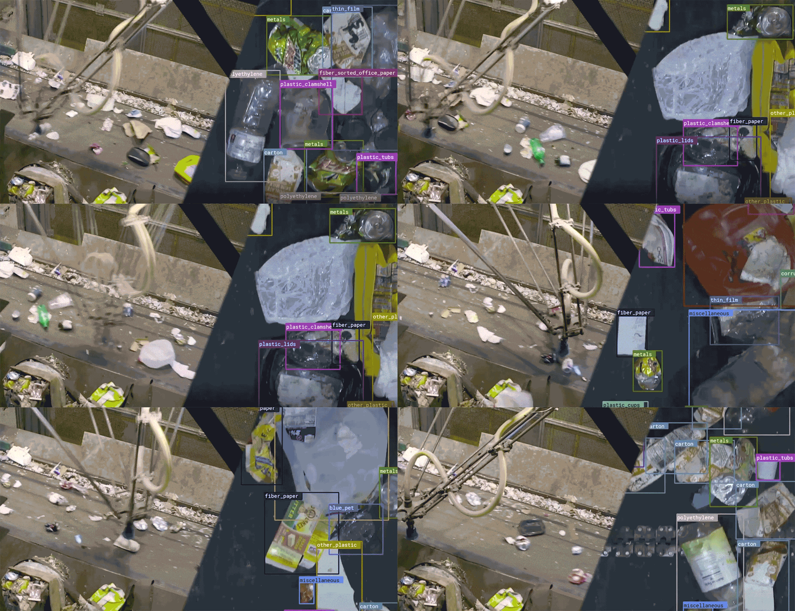
AI-based systems guide robotic arms to grab materials from a stream of mixed recyclables and place them in the correct bins. Here, a tandem robot system operates at a Waste Connections recycling facility [top], and a single robot arm [bottom] recovers a piece of corrugated cardboard. The United States does a pretty good job when it comes to cardboard: In 2021, 91.4 percent of discarded cardboard was recycled, according to the American Forest and Paper Association. AMP Robotics
My company first began using AI in 2016 to extract empty cartons from other recyclables at a facility in Colorado; today, we have systems installed in more than 25 U.S. states and six countries. We weren’t the first company to try AI sorting, but it hadn’t previously been used commercially. And we have steadily expanded the types of recyclables our systems can recognize and sort.
AI makes it theoretically possible to recover all of the recyclables from a mixed-material stream at accuracy approaching 100 percent, entirely based on image analysis. If an AI-based sorting system can see an object, it can accurately sort it.
Consider a particularly challenging material for today’s recycling sorters: high-density polyethylene (HDPE), a plastic commonly used for detergent bottles and milk jugs. (In the United States, Europe, and China, HDPE products are labeled as No. 2 recyclables.) In a system that relies on hyperspectral imaging, batches of HDPE tend to be mixed with other plastics and may have paper or plastic labels, making it difficult for the hyperspectral imagers to detect the underlying object’s chemical composition.
An AI-driven computer-vision system, by contrast, can determine that a bottle is HDPE and not something else by recognizing its packaging. Such a system can also use attributes like color, opacity, and form factor to increase detection accuracy, and even sort by color or specific product, reducing the amount of reprocessing needed. Though the system doesn’t attempt to understand the meaning of words on labels, the words are part of an item’s visual attributes.
We at AMP Robotics have built systems that can do this kind of sorting. In the future, AI systems could also sort by combinations of material and by original use, enabling food-grade materials to be separated from containers that held household cleaners, and paper contaminated with food waste to be separated from clean paper.
Training a neural networkto detect objects in the recycling stream is not easy. It is at least several orders of magnitude more challenging than recognizing faces in a photograph, because there can be a nearly infinite variety of ways that recyclable materials can be deformed, and the systemhas to recognize the permutations.
Inside the Sorting Center
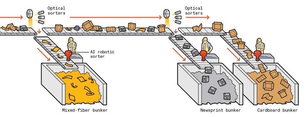
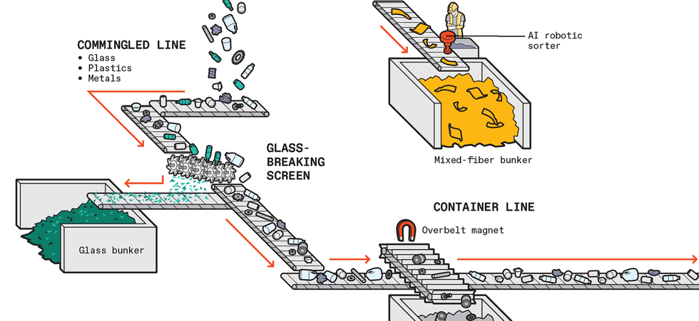
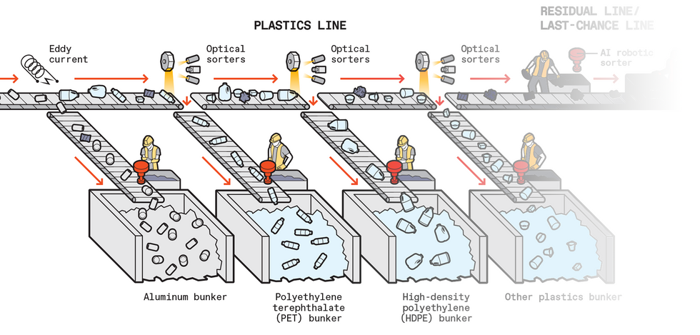
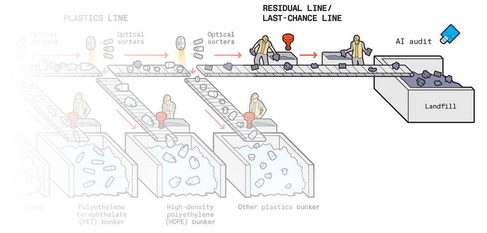
Today’s recycling facilities use mechanical sorting, optical hyperspectral sorting, and human workers. Here’s what typically happens after the recycling truck leaves your house with the contents of your blue bin.
Trucks unload on a concrete pad, called the tip floor. A front-end loader scoops up material in bulk and dumps it onto a conveyor belt, typically at a rate of 30 to 60 tonnes per hour.
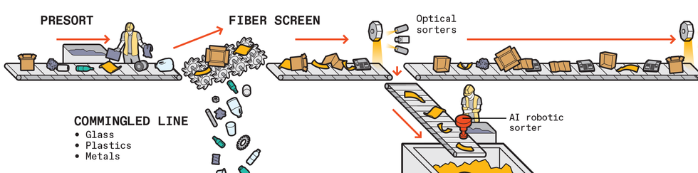
The first stage is the presort. Human workers remove large or problematic items that shouldn’t have made it onto collection trucks in the first place—bicycles, big pieces of plastic film, propane canisters, car transmissions.
Sorting machines that rely on optical hyperspectral imaging or human workers separate fiber (office paper, cardboard, magazines—referred to as 2D products, as they are mostly flat) from the remaining plastics and metals. In the case of the optical sorters, cameras stare down at the material rolling down the conveyor belt, detect an object made of the target substance, and then send a message to activate a bank of electronically controllable solenoids to divert the object into a collection bin.
The nonfiber materials pass through a mechanical system with densely packed camlike wheels. Large items glide past while small items, like that recyclable fork you thoughtfully deposited in your blue bin, slip through, headed straight for landfill—they are just too small to be sorted. Machines also smash glass, which falls to the bottom and is screened out.
The rest of the stream then passes under overhead magnets, which collect items made of ferrous metals, and an eddy-current-inducing machine, which jolts nonferrous metals to another collection area.
At this point, mostly plastics remain. More hyperspectral sorters, in series, can pull off plastics one type—like the HDPE of detergent bottles and the PET of water bottles—at a time.
Finally, whatever is left—between 10 to 30 percent of what came in on the trucks—goes to landfill.
In the future, AI-driven robotic sorting systems and AI inspection systems could replace human workers at most points in this process. In the diagram, red icons indicate where AI-driven robotic systems could replace human workers and a blue icon indicates where an AI auditing system could make a final check on the success of the sorting effort.
It’s hard enough to train a neural network to identify all the different types of bottles of laundry detergent on the market today, but it’s an entirely different challenge when you consider the physical deformations that these objects can undergo by the time they reach a recycling facility. They can be folded, torn, or smashed. Mixed into a stream of other objects, a bottle might have only a corner visible. Fluids or food waste might obscure the material.
We train our systems by giving them images of materials belonging to each category, sourced from recycling facilities around the world. My company now has the world’s largest data set of recyclable material images for use in machine learning.
Using this data, our models learn to identify recyclables in the same way their human counterparts do, by spotting patterns and features that distinguish different materials. We continuously collect random samples from all the facilities that use our systems, and then annotate them, add them to our database, and retrain our neural networks. We also test our networks to find models that perform best on target material and do targeted additional training on materials that our systems have trouble identifying correctly.
In general, neural networks are susceptible to learning the wrong thing. Pictures of cows are associated with milk packaging, which is commonly produced as a fiber carton or HDPE container. But milk products can also be packaged in other plastics; for example, single-serving milk bottles may look like the HDPE of gallon jugs but are usually made from an opaque form of the PET (polyethylene terephthalate) used for water bottles. Cows don’t always mean fiber or HDPE, in other words.
There is also the challenge of staying up to date with the continual changes in consumer packaging. Any mechanism that relies on visual observation to learn associations between packaging and material types will need to consume a steady stream of data to ensure that objects are classified accurately.
But we can get these systems to work. Right now, our systems do really well on certain categories—more than 98 percent accuracy on aluminum cans—and are getting better at distinguishing nuances like color, opacity, and initial use (spotting those food-grade plastics).
Now thatAI-basedsystems are ready to take on your recyclables, how might things change? Certainly, they will boost the use of robotics, which is only minimally used in the recycling industry today. Given the perpetual worker shortage in this dull and dirty business, automation is a path worth taking.
AI can also help us understand how well today’s existing sorting processes are doing and how we can improve them. Today, we have a very crude understanding of the operational efficiency of sorting facilities—we weigh trucks on the way in and weigh the output on the way out. No facility can tell you the purity of the products with any certainty; they only audit quality periodically by breaking open random bales. But if you placed an AI-powered vision system over the inputs and outputs of relevant parts of the sorting process, you’d gain a holistic view of what material is flowing where. This level of scrutiny is just beginning in hundreds of facilities around the world, and it should lead to greater efficiency in recycling operations. Being able to digitize the real-time flow of recyclables with precision and consistency also provides opportunities to better understand which recyclable materials are and are not currently being recycled and then to identify gaps that will allow facilities to improve their recycling systems overall.
Sorting Robot Picking Mixed Plastics AMP Robotics
But to really unleash the power of AI on the recycling process, we need to rethink the entire sorting process. Today, recycling operations typically whittle down the mixed stream of materials to the target material by removing nontarget material—they do a “negative sort,” in other words. Instead, using AI vision systems with robotic pickers, we can perform a “positive sort.” Instead of removing nontarget material, we identify each object in a stream and select the target material.
To be sure, our recovery rate and purity are only as good as our algorithms. Those numbers continue to improve as our systems gain more experience in the world and our training data set continues to grow. We expect to eventually hit purity and recovery rates of 100 percent.
The implications of moving from more mechanical systems to AI are profound. Rather than coarsely sorting to 80 percent purity and then manually cleaning up the stream to 95 percent purity, a facility can reach the target purity on the first pass. And instead of having a unique sorting mechanism handling each type of material, a sorting machine can change targets just by a switch in algorithm.
The use of AI also means that we can recover materials long ignored for economic reasons. Until now, it was only economically viable for facilities to pursue the most abundant, high-value items in the waste stream. But with machine-learning systems that do positive sorting on a wider variety of materials, we can start to capture a greater diversity of material at little or no overhead to the business. That’s good for the planet.
We are beginning to see a few AI-based secondary recycling facilities go into operation, with Amp’s technology first coming online in Denver in late 2020. These systems are currently used where material has already passed through a traditional sort, seeking high-value materials missed or low-value materials that can be sorted in novel ways and therefore find new markets.
Thanks to AI, the industry is beginning to chip away at the mountain of recyclables that end up in landfills each year—a mountain containing billions of tons of recyclables representing billions of dollars lost and nonrenewable resources wasted.
This article appears in the July 2022 print issue as “AI Takes a Dumpster Dive .”
As India’s GDP and per capita income continue to climb, so too will its energy consumption. For instance, just 8 percent of Indian homes had air-conditioning in 2018, but that share is likely to rise to 50 percent by 2050. The country’s electricity consumption in 2019 was nearly six times as great as in 1990. Greenhouse gas emissions will certainly grow too, because India’s energy generation is dominated by fossil fuels—coal-fired power plants for electricity, coal- and gas-fired furnaces for industrial heating, liquid petroleum gas for cooking, and gasoline and diesel for transportation.
Fossil fuels dominate even though renewable energy generation in many parts of the world now costs less than fossil-fuel-based electricity. While electricity from older coal plants in India costs 2.7 U.S. cents per kilowatt-hour and 5.5 cents from newer plants that have additional pollution-control equipment, the cost of solar energy has dropped to 2.7 cents per kilowatt-hour, and wind power to 3.4 cents per kilowatt-hour. As renewable energy has steadily gotten cheaper, the installed capacity has grown, to 110 gigawatts. That amounts to 27 percent of capacity, compared to coal’s share, which is 52 percent. The government of India has set a target of 450 GW of renewable energy capacity by 2030.
Yet in terms of energy generated, renewable energy in India still falls short. In 2021, about 73 percent of the country’s electricity was produced from coal, and only 9.6 percent from solar and wind power. That’s because solar and wind power aren’t available around the clock, so the proportion of the installed capacity that gets used is just 20 to 30 percent. For coal, the capacity utilization rate can go as high as 90 percent.
As renewable energy capacity grows, the only way to drastically reduce coal in the electricity mix is by adding energy storage. Although some of the newer solar plants and wind farms are being set up with large amounts of battery storage, it could be decades before such investments have a significant impact. But there is another way for India to move faster toward its decarbonization goal: by focusing the renewable-energy push in India’s commercial and industrial sectors.
India has some 40,000 commercial complexes, which house offices and research centers as well as shopping centers and restaurants. Together they consume about 8 percent of the country’s electricity. The total footprint of such complexes is expected to triple by 2030, compared to 2010. To attract tenants, the managers of these complexes like to project their properties as users of renewable energy.
A 2-megawatt solar plant located 500 kilometers from IITM Research Park provides dedicated electricity to the complex. A 2.1-MW wind farm now under construction will feed IITMRP through a similar arrangement.IIT Madras
India’s industrial sector, meanwhile, consumes about 40 percent of the country’s electricity, and many industrial operators would also be happy to adopt a greater share of renewable energy if they can see a clear return on investment.
Right now, many of these complexes use rooftop solar, but limited space means they can only get a small share of their energy that way. These same complexes can, however, leverage a special power-transmission and “wheeling” policy that’s offered in India. Under this arrangement, an independent power-generation company sets up solar- or wind-power plants for multiple customers, with each customer investing in the amount of capacity it needs. In India, this approach is known as a group-captive model. The generating station injects the electricity onto the grid, and the same amount is immediately delivered, or wheeled in, to the customer, using the utility’s existing transmission and distribution network. A complex can add energy storage to save any excess electricity for later use. If enough commercial, industrial, and residential complexes adopt this approach, India could rapidly move away from coal-based electricity and meet a greater share of its energy needs with renewable energy. Our group at the Indian Institute of Technology Madras has been developing a pilot to showcase how a commercial complex can benefit from this approach.
The commercial complex known as the IITM Research Park, or IITMRP, in Chennai, is a 110,000-square-meter facility that houses R&D facilities for more than 250 companies, including about 150 startups, and employs about 5,000 workers. It uses an average of 40 megawatt-hours of electricity per weekday, or about 12 gigawatt-hours per year. Within the campus, there is 1 megawatt of rooftop solar, which provides about 10 percent of IITMRP’s energy. The complex is also investing in 2 MW of captive solar and 2.1 MW of captive wind power off-site, the electricity from which will be wheeled in. This will boost the renewable-energy usage to nearly 90 percent in about three years. Should the local power grid fail, the complex has backup diesel generators.
Of course, the generation of solar and wind energy varies from minute to minute, day to day, and season to season. The total generated energy will rarely meet IITMRP’s demand exactly; it will usually either exceed demand or fall short.
To get closer to 100 percent renewable energy, the complex needs to store some of its wind and solar power. To that end, the complex is building two complementary kinds of energy storage. The first is a 2-MWh, 750-volt direct-current lithium-ion battery facility. The second is a chilled-water storage system with a capacity equivalent to about 2.45 MWh. Both systems were designed and fabricated at IITMRP.
The battery system’s stored electricity can be used wherever it’s needed. The chilled-water system serves a specific, yet crucial function: It helps cool the buildings. For commercial complexes in tropical climates like Chennai’s, nearly 40 percent of the energy goes toward air-conditioning, which can be costly. In the IITMRP system, a central heating, ventilation, and air-conditioning (HVAC) system chills water to about 6 °C, which is then circulated to each office. A 300-cubic-meter underground tank stores the chilled water for use within about 6 to 8 hours. That relatively short duration is because the temperature of the chilled water in the tank rises about 1 °C every 2 hours.
The IITMRP’s chilled-water system provides air-conditioning to the complex. Water is chilled to about 6 °C and then stored in this 300-cubic-meter underground tank for later circulation to the offices.IIT Madras
The heat transfer capacity of the chilled-water system is 17,500 megajoules, which as mentioned is equivalent to 2.45 MWh of battery storage. The end-to-end round-trip energy loss is about 5 percent. And unlike with a battery system, you can “charge” and “discharge” the chilled-water tank several times a day without diminishing its life span.
Although energy storage adds to the complex’s capital costs, our calculations show that it ultimately reduces the cost of power. The off-site solar and wind farms are located, respectively, 500 and 600 kilometers from IITMRP. The cost of the power delivered to the complex includes generation (including transmission losses) of 5.14 cents/kWh as well as transmission and distribution charges of 0.89 cents/kWh. In addition, the utilities that supply the solar and wind power impose a charge to cover electricity drawn during times of peak demand. On average, this demand charge is about 1.37 cents/kWh. Thus, the total generation cost for the solar and wind power delivered to IITMRP is about 7.4 cents/kWh.
There’s also a cost associated with energy storage. Because most of the renewable energy coming into the complex will be used immediately, only the excess needs to be stored—about 30 percent of the total, according to our estimate.
So the average cost of round-the-clock renewable energy works out to 9.3 cents/kWh, taking into account the depreciation, financing, and operation costs over the lifetime of the storage. In the future, as the cost of energy storage continues to decline, the average cost will remain close to 9 cents/kWh, even if half of the energy generated goes to storage. And the total energy cost could drop further with declines in interest rates, the cost of solar and wind energy, or transmission and demand charges.
For now, the rate of 9.3 cents/kWh compares quite favorably to what IITMRP pays for regular grid power—about 15 cents/kWh. That means, with careful design, the complex can approach 100 percent renewable energy and still save about a third on the energy costs that it pays today. Keep in mind that grid power in India primarily comes from coal-based generation, so for IITMRP and other commercial complexes, using renewable energy plus storage has a big environmental upside.
IITM Research Park’s lithium-ion battery facility stores excess electricity for use after the sun goes down or when there’s a dip in wind power.IIT Madras
Electricity tariffs are lower for India’s industrial and residential complexes, so the cost advantage of this approach may not be as pronounced in those settings. But renewable energy can also be a selling point for the owners of such complexes—they know many tenants like having their business or home located in a complex that’s green.
Although IITMRP’s annual consumption is about 12 GWh, the energy usage, or load, varies slightly from monthto month, from 970 to 1,100 MWh. Meanwhile, the energy generated from thecaptive off-site solar and wind plants and the rooftop solar plant will vary quite a bit more. Thetop chart ("Monthly Load and Available Renewable Energy at IITMRP") shows the estimated monthly energy generated and the monthly load.
As is apparent, there is some excess energy available in May and July, and an overall energy deficit at other times. In October, November, and December, the deficit is substantial, because wind-power generation tends to be lowest during those months. Averaged over a year, the deficit works out to be 11 percent; the arrangement we’ve described, in other words, will allow IITMRP to obtain 89 percent of its energy from renewables.
For the complex to reach 100 percent renewable energy, it’s imperative that any excess energy be stored and then used later to make up for the renewable energy deficits. When the energy deficits are particularly high, the only way to boost renewable energy usage further will be to add another source of generation, or else add long-term energy storage that’s capable of storing energy over months. Researchers at IITMRP are working on additional sources of renewable energy generation, including ocean, wave, and tidal energy, along with long-term energy storage, such as zinc-air batteries.
IITM Research Park’s electricity load and available renewable energy vary across months [top] and over the course of a single day [bottom]. To make up for the deficit in renewable energy, especially during October, November, and December, additional renewable generation or long-term energy storage will be needed. At other times of the year, the available renewable energy tends to track the load closely throughout the day, with any excess energy sent to storage.
For other times of the year, the complex can get by on a smaller amount of shorter-term storage. How much storage? If we look at the energy generated and the load on an hourly basis over a typical weekday, we see that the total daily load generally matches the total daily demand, but with small fluctuations in surplus and deficit. Those fluctuations represent the amount of energy that has to move in and out of storage. In the bottom chart ("Daily Load and Available Renewable Energy at IITMRP"), the cumulative deficit peaks at 1.15 MWh, and the surplus peaks at 1.47 MWh. Thus, for much of the year, a storage size of 2.62 MWh should ensure that no energy is wasted.
This is a surprisingly modest amount of storage for a complex as large as IITMRP. It’s possible because for much of the year, the load follows a pattern similar to the renewable energy generated. That is, the load peaks during the hours when the sun is out, so most of the solar energy is used directly, with a small amount of excess being stored for use after the sun goes down. The load drops during the evening and at night, when the wind power is enough to meet most of the complex’s demand, with the surplus again going into storage to be used the next day, when demand picks up.
On weekends, the demand is, of course, much less, so more of the excess energy can be stored for later use on weekdays. Eventually, the complex’s lithium-ion battery storage will be expanded to 5 MWh, to take advantage of that energy surplus. The batteries plus the chilled-water system will ensure that enough storage is available to take care of weekday deficits and surpluses most of the time.
As mentioned earlier, India has some 40,000 commercial complexes like IITMRP, and that number is expected to grow rapidly. Deploying energy storage for each complex and wheeling in solar and wind energy make sense both financially and environmentally. Meanwhile, as the cost of energy storage continues to fall, industrial complexes and large residential complexes could be enticed to adopt a similar approach. In a relatively short amount of time—a matter of years, rather than decades—renewable energy usage in India could rise to about 50 percent.
On the way to that admittedly ambitious goal, the country’s power grids will also benefit from the decentralized energy management within these complexes. The complexes will generally meet their own supply and demand, enabling the grid to remain balanced. And, with thousands of complexes each deploying megawatts’ worth of stationary batteries and chilled-water storage, the country’s energy-storage industry will get a big boost. Given the government’s commitment to expanding India’s renewable capacity and usage, the approach we’re piloting at IITMRP will help accelerate the push toward cleaner and greener power for all.
This article appears in the July 2022 print issue as “Weaning India from Coal.”


 Allen Institute on AI et al from FAccT 2022


 Polarized light is an example of superposition. A classical binary digit could be represented by encoding 0 as horizontally (H) polarized light, and 1 as vertically (V) polarized light. Light polarized at other angles has components of both H and V, representing 0 and 1 simultaneously. Examples include the diagonal (D) polarization at 45°, the antidiagonal (A) at –45°, as well as right (R) and left (L) circularly polarized light (the imaginary number i represents a difference in phase). These states become fully fledged quantum bits (qubits) when they consist of pulses that each contain a single photon.
 The possible states of a single isolated qubit [blue arrow] are neatly represented on a sphere, known as a Bloch sphere. The states 0 and 1 sit at the north and south poles, and the polarization states D, A, R, and L lie on the equator. Other possible superpositions of 0 and 1 (described by complex numbers a and b) cover the rest of the surface. Noise can make the qubit state wander continuously from its correct location.
 Simple repetition code [top] on a conventional bit allows single bit-flip errors to be detected via parity checks and then corrected. A similar code for qubits [bottom] must deal with continuous errors. (For simplicity, we depict the case of a logical qubit in a nonsuperposition state, 1.) The parity checks, being quantum measurements, produce discrete outcomes with various probabilities, converting the continuous error into a discrete one and allowing correction by a qubit flip. The individual qubit states are not revealed by the parity measurements.
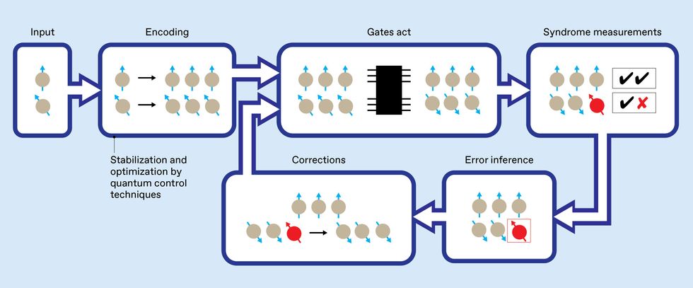 A long quantum computation will require many cycles of quantum error correction (QEC). Each cycle would consist of gates acting on encoded qubits (performing the computation), followed by syndrome measurements from which errors can be inferred, and corrections. The effectiveness of this QEC feedback loop can be greatly enhanced by including quantum-control techniques (represented by the thick blue outline) to stabilize and optimize each of these processes.
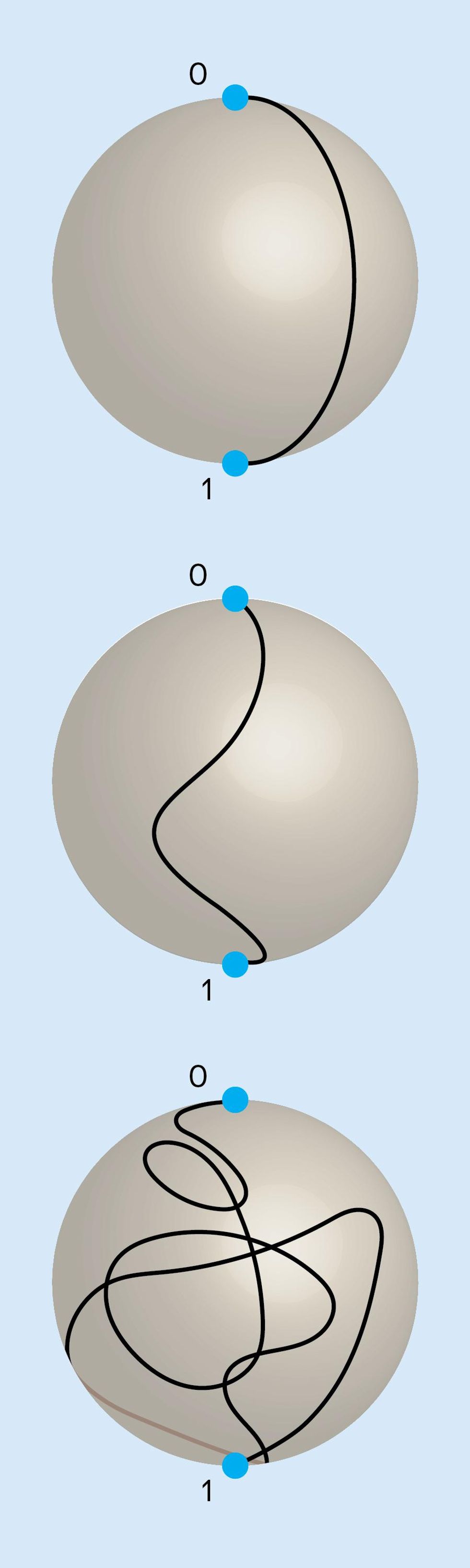 A superconducting qubit can be flipped by applying a simple microwave pulse that takes the qubit’s state on a direct path on the Bloch sphere from 0 to 1 [top], but noise will introduce an error in the final position. A complicated pulse producing a more circuitous route can reduce the average amount of error in the final position. Here,



 AMP Robotics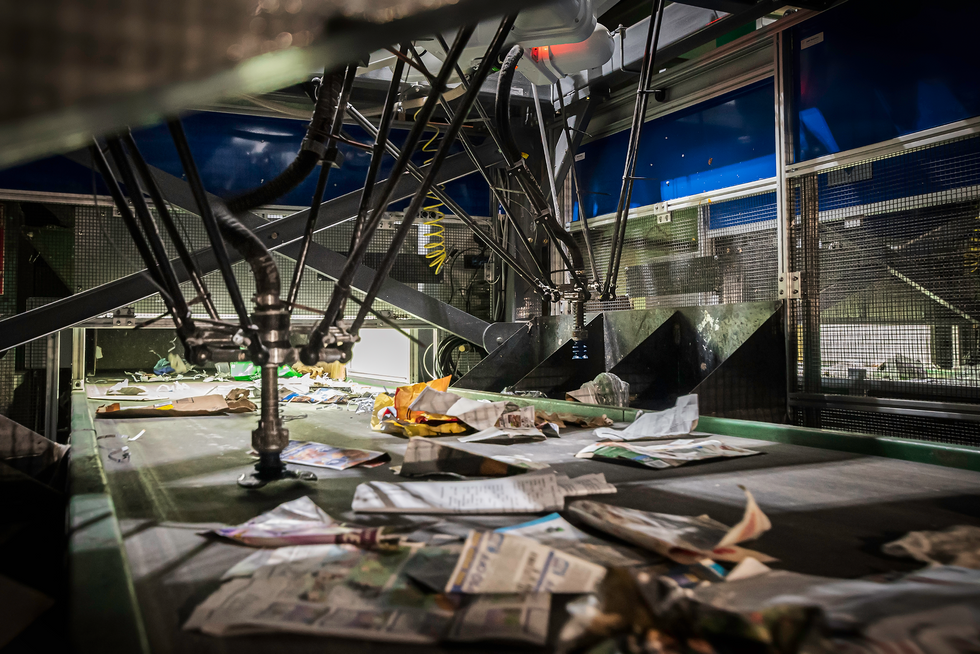
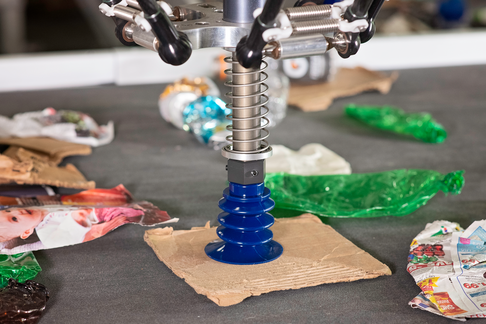 AI-based systems guide robotic arms to grab materials from a stream of mixed recyclables and place them in the correct bins. Here, a tandem robot system operates at a Waste Connections recycling facility [top], and a single robot arm [bottom] recovers a piece of corrugated cardboard. The United States does a pretty good job when it comes to cardboard: In 2021, 91.4 percent of discarded cardboard was recycled, according to the American Forest and Paper Association. AMP Robotics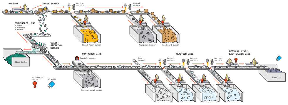
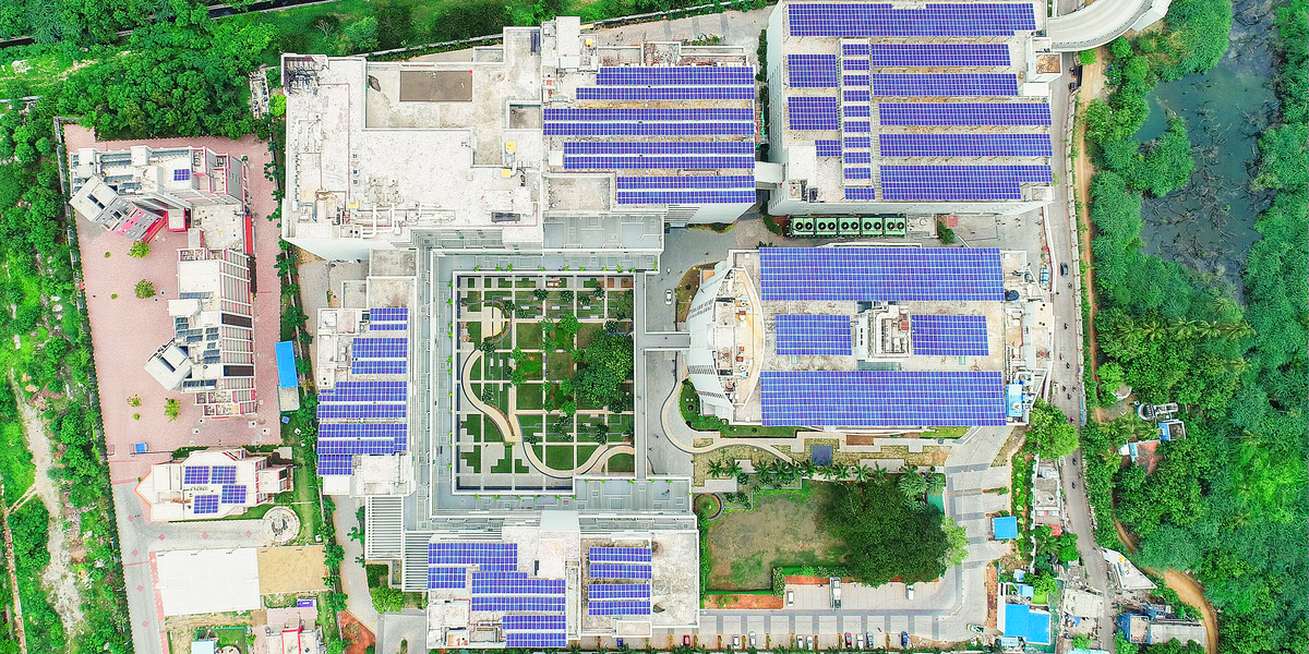

 A 2-megawatt solar plant located 500 kilometers from IITM Research Park provides dedicated electricity to the complex. A 2.1-MW wind farm now under construction will feed IITMRP through a similar arrangement.IIT Madras
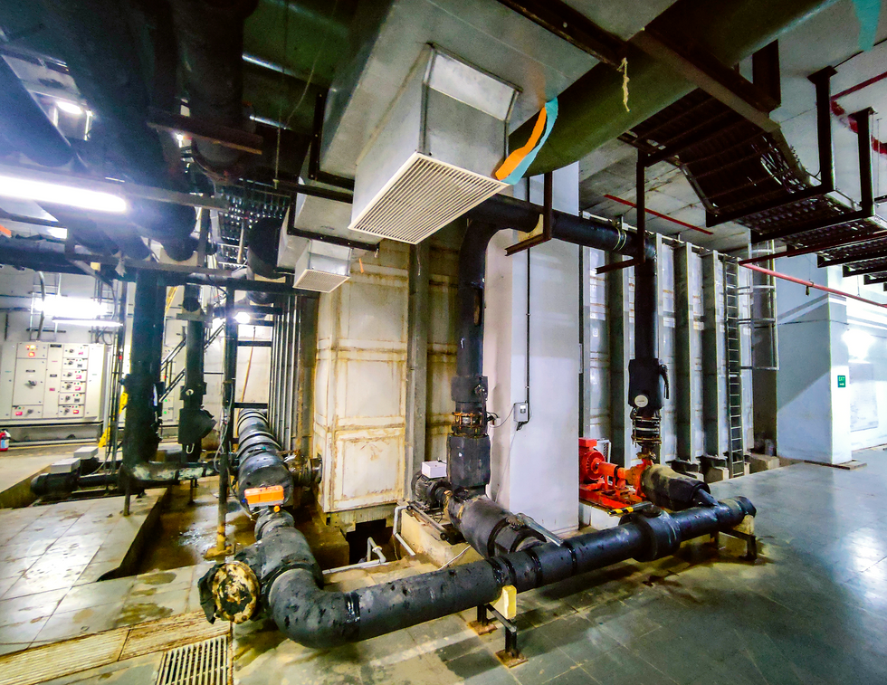 The IITMRP’s chilled-water system provides air-conditioning to the complex. Water is chilled to about 6 °C and then stored in this 300-cubic-meter underground tank for later circulation to the offices.IIT Madras
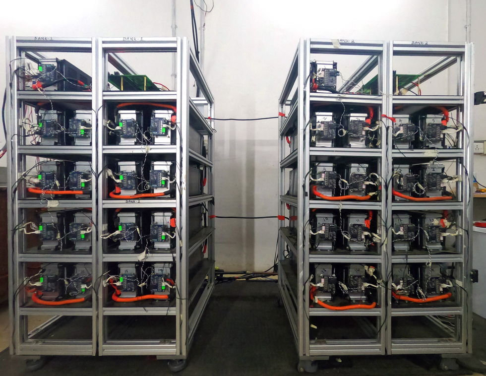 IITM Research Park’s lithium-ion battery facility stores excess electricity for use after the sun goes down or when there’s a dip in wind power.IIT Madras


